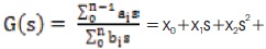
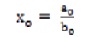
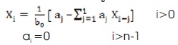
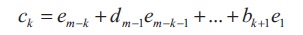
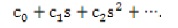
The coefficients of the power series expansion given as,
The mth reduced order model is,
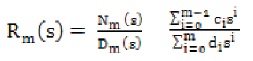
Here Dm(s) is known through equations, Nm(s) of pade approximation of G(s) is,
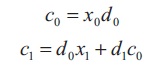

The coefficients ci ; i=0, 1, 2,...m-1 can be found by solving m linear equations in Equation (5).
Consider the Taylor series expansion of the impulse response of the higher order system.
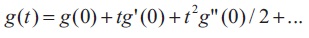
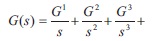
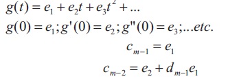
The values of g(0), g’(0), ... etc., are very simply related to the parameters of the transfer function G(s). Expanding G(s) in an infinite series in powers of s-1 , gives,
and taking inverse Laplace transforms of it gives,
assuming k is positive.
The drawback of the pade approximation method is that the poles of the reduced order system depend on both the numerator and the denominator of the original transfer function, and hence may result in an unstable approximate for a stable system ( Kumar et al., 2019).
1.2. Routh Approximation
This method has been proposed by Hutton and Friedland (1975). In this method, first Routh table is developed for the original system and then coefficients of its Routh table calculated in such a manner that it agree with the original system. This ensures system stability and the steady state values of reduced order models which match with the original system. This method involves simple algebraic calculation of finite number of steps. The general rational function i.e., the difference between numerator and denominator order not less than one can also be reduced by slight modification in the beta table proposed in Routh approximates of arbitrary order. This method can be applied to both time and frequency domain but lacks in flexibility when the reduced order model does not produce a good approximation (Prajapati & Prasad, 2018; Prasad, 2000).
1.3 Routh-Pade Mixed Approximation
Due to drawbacks in Routh approximation, a mixed approach is used for finding stable reduced-order models using the Pade approximation technique and the Routh- Hurwitz array ( Shamash, 1975). This approach ensures reduced model stability where the original system is stable.
It is computationally easy to program and conceptually simple. Mixed technique combines the Pade approximation and the Routh-Hurwitz array method ( Sikander & Prasad, 2015).
Let the higher order transfer function H(s) be given by,
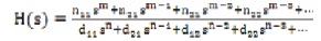
where m < n and Equation (2) is the power series expansion of Equation (9) about s = 0.
Step1: Routh-Hurwitz stability array is formed for the denominator polynomial in Equation (9).
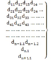
The above array is formed by the well-known algorithm,
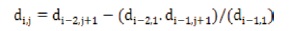
for i ≥ 3 and 1≤ j ≤ [(– i + 3)/2], where [ ] stands for the integral part of the quantity. The transfer function of reduced order k may be written as,
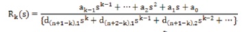
where the coefficients of the k order denominator polynomial are found from Equation (12). R k(s) may be rewritten as,
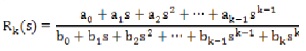
where the b coefficients are now known.
Step 2: For numerator coefficient a0 , a1 ……ak-1 can be found as mentioned in Pade approximation.
2. Numerical Example
In this paper, Pade approximation and Routh-Pade approximation methods are used for order reduction, time domain and frequency domain characteristics of reduced model is compare with the previous obtained methods.
Example: Consider a fourth-order system ( Parmar et al., 2007), represented by the following transfer function.
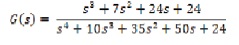
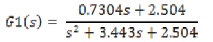
The transfer function of required second-order reduced model by pade approximation method is obtained as,
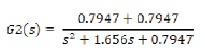
By Routh-Pade approximation, reduced model is obtained as,
The step response curve has been drawn as shown in Figure 1 and Figure 2.
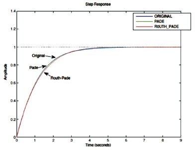
Figure 1. Comparison of Step Response of Original with Pade, Routh-Pade Reduced Order Model
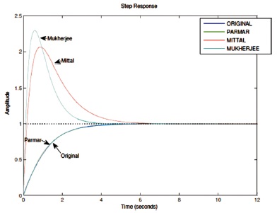
Figure 2. Comparision of Step Response of Orginal with Previous Reduced Order Model
3. Result and Discussion
In this paper, denominator polynomial is obtained through Routh-Pade approximation and numerator polynomial through Pade approximation for fourth order system. Comparison of step response of original with Pade, Routh- Pade reduced order model is shown in Figure 1. The transient response parameter of original system is compared with different reduced order model as mentioned in Table 1. It is clear from the Table 1 that dominant pole is preserved in Pade, Parmar et al. (2007) and Mittal et al. (2004) methods. Pade approximation method has same rise time, settling time as in original system. Mittal et al. (2004) and Mukherjee and Mishra (1987) show large deviation in time domain characteristics while steady state behaviour is maintained in Parmar et al. (2007). The matching of the step response is comparatively better in Pade, Routh-Pade, Parmar et al. (2007), while Mittal et al. (2004) and Parmar et al. (2007) model have large overshoot as shown in Figure 2. A frequency domain characteristics of the original system is compared with various reduced order model in Table 2. Comparison of frequency domain characteristics of original with reduced order model is shown in Figure 3. Mittal et al. (2004) and Mukherjee and Mishra (1987) model shows large deviation from original model frequency domain characteristics.
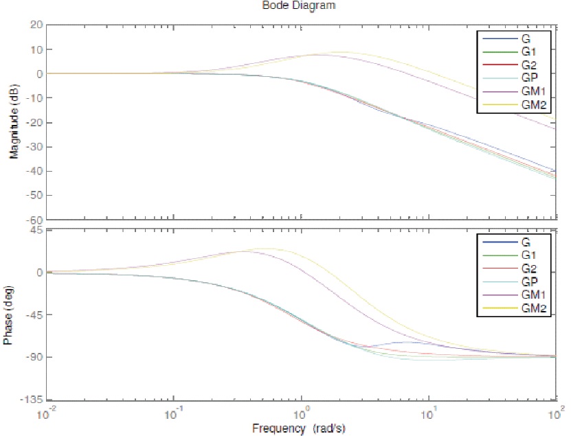
Figure 3. Comparison of Frequency Domain Characteristics of Original with Reduced Order Model
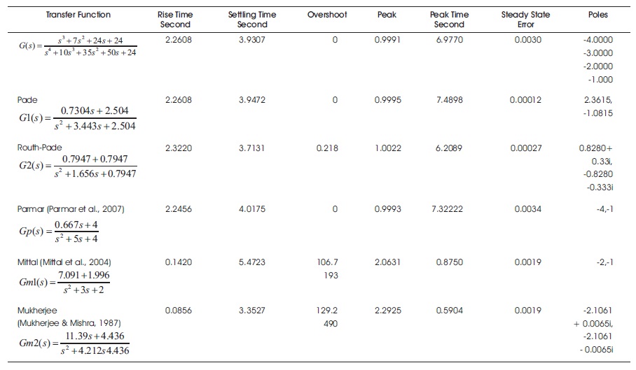
Table 1. Comparison of Time Domain Specification of Reduced Order Models Obtained through Proposed and Other Methods for Example
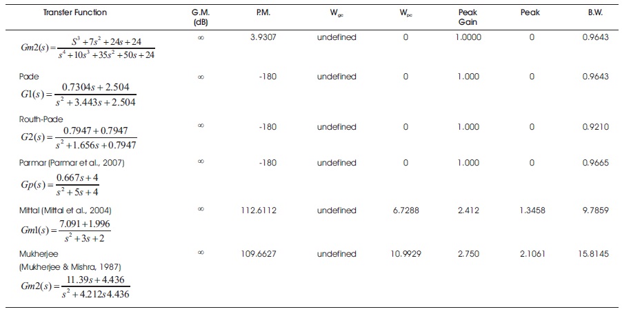
Table 2. Comparison of Frequency Domain Specification of Reduced Order Models Obtained through Proposed and Other Methods
Conclusion
The study of the original system and its reduced models is being carried out. The systems are subjected to step input and the response is analyzed in time domain and frequency domain. It clearly shows that the proposed method gives better result. The steady state error is compared for the proposed and the other well-known existing order reduction techniques. From the results it is clear that the proposed algorithm gives low value of the steady state error in frequency domain.